Visualizing linear algebra: Dot product

Figure 1: Column vector as an arrow

This is Part 5 in a series on linear algebra [1].

Figure 1 shows a vector that is represented geometrically as a yellow arrow and numerically as a column. It scales the unit vectors i-hat and j-hat by 2 and 4 respectively. That is:

v = 2î + 4ĵ

Now suppose the column is transposed to a row, as follows:

[2]^T = [2 4]
[4]

This row is a 2x1 matrix that represents the transformation of a 2D vector space to a 1D vector space, that is, a number line. The number line is the span of the yellow arrow (i.e., it extends along the yellow arrow in both directions).

Figure 2: Row vector as a transformation matrix

The effect of this transformation on the unit vectors is shown in Figure 2 where i-hat is scaled by 2 and j-hat is scaled by 4. The length of the yellow arrow, per Pythagoras' Theorem, is √(2² + 4²) =  √20, or about 4.47.

For any given input vector, the position on the number line where the input vector ends up will be the vector's X coordinate scaled by 2 plus the vector's Y coordinate scaled by 4.

Figure 3: Calculating the dot product

For example, the purple arrow in Figure 3 is transformed to a 1D vector, or scalar, on the number line as follows:

[2 4][2] = 2[2] + 1[4] = 8
     [1]

Geometrically, this is equivalent to projecting the purple arrow onto the span of the yellow arrow (at position 8/√20, or 1.79) and scaling by the length of the yellow arrow (√20, or 4.47). The small right-angled triangle in Figure 3 shows the projection.

In the symmetrical example where the column for the purple arrow is transposed to a row (representing a transformation to the number line that is the span of the purple arrow), the yellow arrow is transformed as follows:

[2 1][2] = 2[2] + 4[1] = 8
     [4]

The scalar result is the same as for the first example - the vector order doesn't matter. However geometrically, it is equivalent to projecting the yellow arrow onto the span of the purple arrow (at position 8/√5, or 3.58) and scaling by the the length of the purple arrow (√(2² + 1²) =  √5, or 2.24). The large right-angled triangle in Figure 3 shows the projection.

More generally, this operation is the dot product (or scalar product) of two vectors and for 2D vectors is defined [2] as:

a.b = a_xb_x + a_yb_y

When the arrows are pointing in the same general direction the dot product is positive, when pointing in the opposite direction the dot product is negative, and when the arrows are orthogonal the dot product is zero.

Figure 4: Dot product = transform

Numerically the dot product multiplies two vectors, taking direction into account [3].

Geometrically, one vector encodes a linear transformation that projects space onto a number line and scales the projection by the length of the vector.

Next up: the cross product

--

[1] The figures and examples of the posts in this series are based on the Essence of Linear Algebra series by 3Blue1Brown.

[2] The dot product is also defined as

a.b = ∥a∥∥b∥cos(θ)

where ∥v∥ denotes the magnitude of vector v. This can also be interpreted as projecting one of the vectors onto the other vector (via the cosine) and scaling by the other vector.

[3] The numerical summary comes from Better Explained which also offers further analogies.

Visualizing linear algebra: Matrix inverse

Figure 1: A linear system of equations

This is Part 4 in a series on linear algebra [1].

In the series so far, matrices have been used to transform a vector space. This is particularly useful for applications such as computer graphics and robotics. However its most general use is in the solving of linear systems of equations. In a linear equation, the only thing happening to each variable is that it is being scaled by some constant. And the only thing happening to each of those scaled variables is that they are added to each other.

Figure 1 shows two linear equations. These two equations are packaged into a single vector equation where the 2x2 matrix A contains all the constant coefficients, vector x contains the variables x and y, and vector v contains the constants. Per the equation itself, vector x multiplied by matrix A equals the vector v.

Matrix A represents a linear transformation, so solving Ax = v means we're looking for a vector x which, after applying the transformation to it, lands on vector v. The way to find vector x is by applying the transformation in reverse. That is, when the inverse transformation is applied to vector v, vector v will end up landing on vector x. The inverse of A is represented as A^-1. AA^-1 = A^-1A = I, where I is the identity matrix [2]. Geometrically, applying a transformation to a vector space and then applying the inverse transformation restores the original vector space. This is equivalent to applying the identity matrix which leaves the vector space unchanged. The identity (or unit) matrix is defined as:

[1 0]
[0 1]

Notice that the identity matrix columns are simply the unit vectors i-hat and j-hat. Now multiplying both sides of the equation Ax = v by A^-1 results in the equation A^-1Ax = Ix = x = A^-1v.

The equation for calculating the inverse of a matrix is:

[a b]^-1 = 1/(ad - bc)[ d -b]
[c d]                [-c  a]

Note that the determinant of the matrix appears in the expression (ad - bc). There will be an inverse matrix as long as the determinant is non-zero. Calculating A^-1:

[2 2]^-1 = 1/(2*3 - 2*1)[ 3 -2] = 1/4[ 3 -2]
[1 3]                  [-1  2]      [-1  2]

Figure 2: Solving the equations

Solving our vector equation:

x = A^-1v
  = 1/4[ 3 -2][-4]
       [-1  2][-1]
  = 1/4*(-4[ 3] + -1*[-2])
           [-1]      [-2]
  = 1/4[-4* 3 + -1*-2]
       [-4*-1 + -1* 2]
  = 1/4[-10]
       [  2]
  = [-2.5]
    [ 0.5]

Plugging x and y into the original linear equations:

2x + 2y = 2 * -2.5 + 2 * 0.5 = -5 + 1 = -4
1x + 3y = 1 * -2.5 + 3 * 0.5 = -2.5 + 1.5 = -1

That confirms that the correct solution has been found. Figure 2 shows the geometric representation of the vector equation.

The set of all possible outputs for a matrix, whether a plane, a line, a 3D space, and so on, is called the column space of the matrix (the span of the columns). The number of dimensions in the column space of a matrix is its rank. In the above example, the rank is two (and, since the determinant is non-zero, the matrix is full rank). If the determinant is zero and the area reduces to a line or point, then the rank is one or zero respectively. Solutions only exist in the rank one case if the vector falls on the line. The zero vector is included in the column space and the set of vectors that land on the origin is called the null space or kernel of a matrix.

Next up: the dot product

--

[1] The figures and examples of the posts in this series are based on the Essence of Linear Algebra series by 3Blue1Brown.

[2] The inverse of a matrix is analogous to the reciprocal of a number. Just as 8*8^-1 = 1, so AA^-1 = I, where I is the identity matrix (itself analogous to the number 1).

Visualizing linear algebra: Determinant

Figure 1: The determinant of the unit matrix is 1

This is Part 3 in a series on linear algebra [1].

Consider the 1x1 unit square in Figure 1 whose sides are circumscribed by i-hat and j-hat. When a linear transformation is applied to the vector space, the unit square is transformed into a parallelogram. The factor by which the transformation scales the area is called the determinant of that transformation.

Figure 2: The determinant of any matrix is ad - bc

The equation for calculating the determinant is

det([a b]) = ad - bc

    [c d]

The determinant is a measure of the area of a parallelogram. However in the cases where i-hat switches to the left of j-hat, the determinant will be negative. This can be understood geometrically as the flipping of the area, like turning over a piece of paper (i.e., inverting the matrix).

Some transformations will result in i-hat and j-hat ending up on the same line, in which case the area and thus the determinant will be 0.

Figure 2 shows how the equation is derived. Breaking it down:

det([a b]) = (a + b)(c + d) - ac - bd - 2bc = ad - bc

    [c d]

The calculation takes the area of the rectangle circumscribing the parallelogram and then just subtracts the areas of the smaller squares and triangles surrounding the parallelogram.

When either b or c are equal to 0, the area will just be ad. This corresponds to when either i-hat or j-hat remain on their original axes. That is, when the final shape is either a rectangle (in the case of both b and c being 0) or a shear along just one dimension.

Figure 3:The determinant of this flipped area is -3

Working through some examples, the matrix in Figure 3 is

[1  2]
[1 -1]

The determinant is

ad - bc = 1*-1 - 2*1 = -3

Note that i-hat ends up to the left of j-hat which means the orientation of space has been inverted resulting in a negative determinant.

Figure 4: The determinant of a line is 0

The matrix in Figure 4 is

[4 2]
[2 1]

The determinant is

ad - bc = 4*1 - 2*2 = 0

Note that i-hat ends up on the same line as j-hat (i.e., the matrix columns are linearly dependent) which means the determinant must be 0. A matrix with a determinant of 0 is also termed a degenerate or non-invertible matrix.

Figure 5: A parallelepiped

The determinant can also be calculated for square matrices that are three dimensional or higher. In the case of a 3x3 matrix, the determinant is a measure of the volume of a parallelepiped and the equation is

det([a b c])

    [d e f]  = a det([e f]) 

    [g h i]          [g h]

             - b det([d f])

                     [h i]

             + c det([d e])

                     [g i]

The determinant will be negative when the 3D space is inverted which can be determined visually using the right-hand-rule. A determinant of 0 would mean that the space is transformed to a lower dimensional space with zero volume and so would be either a plane, a line, or a point. In this special case, the columns of the matrix are linearly dependent.

Next up: the inverse of a matrix

--

[1] The figures and examples of the posts in this series are based on the Essence of Linear Algebra series by 3Blue1Brown.

Visualizing linear algebra: Matrices

"Unfortunately, no one can be told what the Matrix is.
You have to see it for yourself." - Morpheus

This is Part 2 in a series on linear algebra [1].

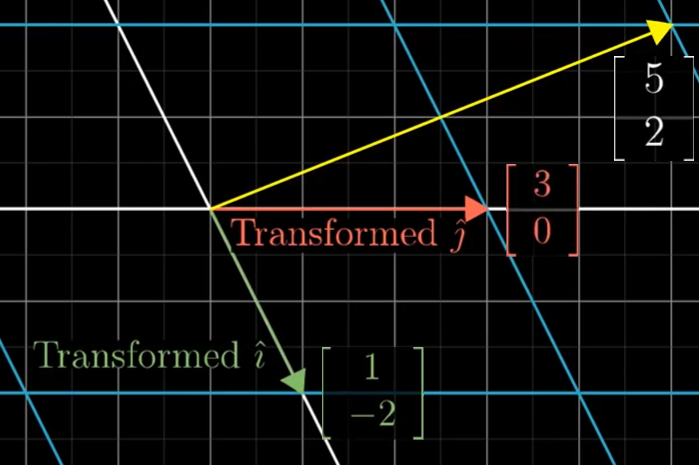
A vector can be visualized as an arrow in space and any given vector is the linear combination of the scaled unit vectors [2]:

v = xî + yĵ

A 2 x 2 matrix represents a linear transformation of the original 2D vector space which might be a rotation or a shear or a more complex transformation (as long as vectors remain straight and fixed to the origin).

Figure 1: Before transformation of the vector space

For example, consider the matrix

[ 1 3]
[-2 0]

The matrix encodes two column vectors that specify where the two unit vectors (î and ĵ) end up when the vector space is transformed.

Figure 1 shows the two unit vectors (î and ĵ) before the linear transformation and Figure 2 shows the effect of the transformation on those two vectors.

Figure 2: After transformation of the vector space

To find out where any given vector ends up, simply multiply the vector by the matrix.

Consider the yellow arrow in Figure 1 which is represented by the vector

[-1]
[ 2]

Figure 2 shows the effect of the linear transformation on the yellow arrow. In numerical terms, the vector is multiplied by the matrix as follows [3]:

[ 1 3][-1] = -1[ 1] + 2[3] = [-1* 1 + 2*3] = [5]
[-2 0][ 2]     [-2]    [0]   [-1*-2 + 2*0]   [2]

So the place where the vector ends up is -1 times the vector where i-hat ends up plus 2 times the vector where j-hat ends up. That is, the vector started off as a specific linear combination of i-hat and j-hat (-1î + 2ĵ) and it ended up as that same linear combination of where those two unit vectors ended up.

To summarize, a vector is an arrow in space and a matrix is a linear transformation of that space (say, a rotation). So to visualize the arrow in the transformed space, just multiply the vector by the matrix.

Figure 3: Rotate counterclockwise then shear right

It is also possible to apply multiple transformations in succession. In Figure 3, the original vector space is rotated then sheared. The overall effect is another linear transformation, called a composition, that is distinct from the rotation and the shear. The composition (or product) matrix can be calculated by multiplying the rotation matrix by the shear matrix, as follows:

[1 1][0 -1] = [1 -1]
[0 1][1  0]   [1  0]

Note that the first column of the composition matrix shows where i-hat ends up and the second column shows where j-hat ends up. Also note the right-to-left rule [3], so the rotation (blue) occurs first and is then followed by the shear (purple). Order matters, since a shear followed by a rotation would produce a different composition matrix (i.e., the green arrow would end up pointing in a north-west direction). Generally:

[i_x2 j_x2][i_x1 j_x1] = [i_x1i_x2 + i_y1j_x2   j_x1i_x2 + j_y1j_x2]
[i_y2 j_y2][i_y1 j_y1]   [i_x1i_y2 + i_y1j_y2   j_x1i_y2 + j_y1j_y2]

Breaking this down, i and j represent the columns where i-hat and j-hat end up for each matrix. So to calculate where i-hat and j-hat end up in the composition matrix, i and j in the first (blue) matrix each have to be transformed (multiplied) by the second (purple) matrix. So calculating where i-hat ends up first:

[i_x2 j_x2][i_x1] = i_x1[i_x2] + i_y1[j_x2] = [i_x1i_x2 + i_y1j_x2]
[i_y2 j_y2][i_y1]      [i_y2]      [j_y2]   [i_x1i_y2 + i_y1j_y2]

The transformed i-hat vector is the first column of the composition matrix. Similarly calculating where j-hat ends up:

[i_x2 j_x2][j_x1] = j_x1[i_x2] + j_y1[j_x2] = [j_x1i_x2 + j_y1j_x2]
[i_y2 j_y2][j_y1]      [i_y2]      [j_y2]   [j_x1i_y2 + j_y1j_y2]

The transformed j-hat vector is the second column of the composition matrix.

The final effect is that i-hat and j-hat are transformed as indicated by the two columns in the composition matrix. In this way, any number of transformations can be combined in the desired order to produce a new composition matrix.

Consider again the composition of the rotation and shear above. To visualize an arrow in the transformed space, just multiply the vector by the composition matrix. As shown above, the effect is exactly the same as applying the rotation then the shear, except that those two actions are applied in a single action. That is:

[1 1][0 -1][x] = [1 -1][x]
[0 1][1  0][y]   [1  0][y]

It is also possible to represent a transformation between dimensions. A matrix with 3 rows by 2 columns represents a 2D to 3D transformation, whereas a matrix with 2 rows by 3 columns represents a 3D to 2D transformation.

Next up: the determinant of a matrix

--

[1] The figures and examples of the posts in this series are based on the Essence of Linear Algebra series by 3Blue1Brown.

[2] Recall the unit vectors, where î (i-hat) is the arrow of unit length along the X-axis and ĵ (j-hat) is the arrow of unit length along the Y-axis.

Figure 4: Unit vectors

[3] Note that vectors and matrices are multiplied from right to left. The reason for this is that matrices are essentially functions. In function notation, the function M₂(M₁(V)) calculates from inner to outer which, visually, is from right to left. Note also that the order matters because matrix multiplication is non-commutative. That is M₁M₂ != M₂M₁.

Visualizing linear algebra: Vectors

Figure 1: Numeric and geometric
representation of a 2D vector

This is Part 1 in a series on linear algebra [1].

Geometrically, a vector is an arrow that has two components: a length and a direction. The yellow arrow in Figure 1 lives in a 2D vector space defined by a horizontal (X) dimension and a vertical (Y) dimension and with the tail of the arrow at the origin.

An equivalent numeric representation is as an ordered list of numbers. As shown in Figure 1, the column stores the coordinates of the vector from top to bottom in order of dimension (i.e., X then Y). A 2D vector can be represented generally as:

[x]
[y]

Figure 2: Vector addition

Vectors, like numbers, can be added. Geometrically, considering the two vectors that are to be added as arrows, this is done by moving the second arrow such that its tail is at the head of the first arrow. The sum is itself an arrow which extends from the tail of the first arrow to the head of the second arrow. In Figure 2, the summed arrow is represented by the purple arrow extending from the origin.

In the numeric representation, the sum vector is calculated by adding the coordinates for each dimension. Generally:

[x₁] + [x₂] = [x₁ + x₂]
[y₁]   [y₂]   [y₁ + y₂]

Figure 3: Vector multiplication (scaling)

Vectors can also be multiplied by a number. This number is called a scalar since it scales the vector by that number. In Figure 3, the original arrow is scaled by 2.

In the numeric representation, the product vector is calculated by multiplying each coordinate by the scalar. Generally:

s * [x] = [s * x]
    [y]   [s * y]

Figure 4: Linear combination of scaled unit vectors

In a 2D coordinate system there are two special vectors: i-hat (î) is the unit vector in the horizontal (X) direction and j-hat (ĵ) is the unit vector in the vertical (Y) direction.

Each of the coordinates in any given vector can be considered as scalars that scale the unit vectors. In Figure 4, i-hat is flipped (since the scalar is negative) and scaled by a factor of 5 while j-hat is scaled by a factor of 2. That is, the yellow arrow is the sum of the two scaled unit arrows.

When any vectors are scaled and added in this way, the resulting expression is a linear combination of those scaled unit vectors (which is, itself, a vector as geometrically represented by the yellow arrow in Figure 4). Generally:

v = xî + yĵ

The span of the unit vectors is the 2D plane (the set of all their possible linear combinations). That is, any point on the 2D plane can be reached by a unique scaling of the two unit vectors. This is also true for most pairs of vectors except those that reside on the same line (in which case their span is just the 1D line and so these vectors are linearly dependent). The unit vectors are linearly independent and, for simplicity, are often chosen as the basis vectors for a 2D space as in Figure 4. This general idea also extends to three and higher dimensions where, for example, the span of the three unit vectors is the 3D volume.

Next up: matrices

--

[1] The figures and examples of the posts in this series are based on the Essence of Linear Algebra series by 3Blue1Brown.

What does science say about sexual orientation?

Sexual orientation: biology or choice?

The scientific research regarding sexual orientation has ongoing political, religious and social implications. This post highlights the specifically scientific conclusions on the causes of sexual orientation. I've structured it in a Question and Answer format with quotes from the relevant scientific literature.

In particular, a comprehensive meta-analysis study conducted by J. Michael Bailey and colleagues in the journal Psychological Science in the Public Interest in 2016 is referenced which provides a systematic review of the scientific research.

What percentage of people have a same-sex attraction?

From the 2016 meta-analysis study:

"Those with predominantly same-sex attractions comprise fewer than 5% of respondents in most Western surveys. Data from non-Western cultures are consistent with this conclusion. There is no persuasive evidence that the rate of same-sex attraction has varied much across time or place." [1]

What causes one's sexual orientation?

From the 2016 meta-analysis study:

"No causal theory of sexual orientation has yet gained widespread support. The most scientifically plausible causal hypotheses are difficult to test. However, there is considerably more evidence supporting nonsocial causes of sexual orientation than social causes. This evidence includes the cross-culturally robust finding that adult homosexuality is strongly related to childhood gender nonconformity; moderate genetic influences demonstrated in well-sampled twin studies; the cross-culturally robust fraternal-birth-order effect on male sexual orientation; and the finding that when infant boys are surgically and socially “changed” into girls, their eventual sexual orientation is unchanged (i.e., they remain sexually attracted to females). In contrast, evidence for the most commonly hypothesized social causes of homosexuality—sexual recruitment by homosexual adults, patterns of disordered parenting, or the influence of homosexual parents—is generally weak in magnitude and distorted by numerous confounding factors." [1]

To elaborate on the above nonsocial causes:

1. Childhood gender nonconformity: "Behaving like the other sex—is a strong correlate of adult sexual orientation that has been consistently and repeatedly replicated." [1]
2. Moderate genetic influences demonstrated in well-sampled twin studies: "Twin siblings of homosexual males are more likely to be homosexual than non-twin siblings." [4]
3. The cross-culturally robust fraternal-birth-order effect on male sexual orientation: "The number of biological older brothers, including those not reared with the participant (but not the number of nonbiological older brothers), increases the probability of homosexuality in men. These results provide evidence that a prenatal mechanism(s), and not social and/or rearing factors, affects men’s sexual orientation development." [4]
4. When infant boys are surgically and socially “changed” into girls, their eventual sexual orientation is unchanged (i.e., they remain sexually attracted to females): "These results comprise the most valuable currently available data concerning the broad nature-versus-nurture question for sexual orientation. They show how difficult it is to derail the development of male sexual orientation by psychosocial means." [1]

From Wikipedia:

"Biological theories for explaining the causes of sexual orientation are favored by scientists and involve a complex interplay of genetic factors, the early uterine environment and brain structure. These factors, which may be related to the development of a heterosexual, homosexual, bisexual, or asexual orientation, include genes, prenatal hormones, and brain structure." [2][3]

What are the relevant peer-reviewed scientific studies?

• The 2016 meta-analysis has a comprehensive survey of the scientific research [1].
• A summary of 19 peer-reviewed studies relevant to the question Is sexual orientation determined at birth? Of the 19 studies, 15 conclude in the affirmative, one in the negative and three are non-conclusive. [4]

Is the presence of same sex orientation in the population a Darwinian paradox?

From Australia’s Science Channel:

"Jenny Graves, professor of genetics at LaTrobe University in Melbourne, has no problem with the concept of gay genes.

'The idea that a person’s genetic makeup affects their mating preference is unsurprising,' she writes in The Conversation. 'We see it in the animal world all the time. There are probably many genes that affect human sexual orientation.'

But rather than thinking of them as 'gay genes', perhaps, she says, we should consider them “male-loving genes”.

'They may be common because these variant genes, in a female, predispose her to mate earlier and more often, and to have more children.'

Graves cites an Italian study [5] that shows female relatives of gay men having 1.3 times as many children as the female relatives of straight men. One possible explanation is that “male-loving” alleles – our gene variants – in a female they predispose her to mate earlier and have more children, so making up for the fewer children of gay males." [6]

References:

[1] "Sexual Orientation, Controversy, and Science", Psychological Science in the Public Interest, 2016.

[2] https://en.wikipedia.org/wiki/Biology_and_sexual_orientation

[3] https://en.wikipedia.org/wiki/Sexual_orientation

[4] Peer-Reviewed Studies on the Origin of Sexual Orientation Since 1990

[5] "Evidence for maternally inherited factors favouring male homosexuality and promoting female fecundity", Proceedings, Biological Sciences, 2004

[6] https://australiascience.tv/science-of-sexuality/

The liar paradox (Part 2)

In my previous post I discussed the liar paradox and argued that it should not be considered either true or false because it is cyclic. That is, it never ends up successfully asserting anything about the world.

Interestingly, the Stanford Encyclopedia of Philosophy (SEP) entry for the Liar Paradox outlines an argument that the liar sentence implies a contradiction. The argument uses two inference rules, as follows:

• Capture: A implies "A" is true
• Release: "A" is true implies A

Taking these two rules together, the terms A and "A" is true are intersubstitutable [1]. The SEP argument, reproduced in plain English [2], is:

Let L be the sentence, "This sentence is not true".

    1. "L" is true or "L" is not true [Law of Excluded Middle]
    2. Case One:
         a. "L" is true
         b. L [2a: release]
         c. "L" is not true [2b: definition of L]
         d. "L" is true and "L" is not true [2a, 2c: conjunction introduction]
    3. Case Two:
         a. "L" is not true
         b. L [3a: definition of L]
         c. "L" is true [3b: capture]
         d. "L" is true and "L" is not true [3a, 3c: conjunction introduction]
    4. "L" is true and "L" is not true [1-3: disjunction elimination]

Line 1 assumes that the liar sentence conforms to the Law of Excluded Middle. That is, it assumes that the liar sentence is either true or not true and not some other value. Lines 2 and 3 analyze each disjunct as separate cases. In each case a contradiction is reached which is then inferred in 4.

The conclusion that the liar sentence implies a contradiction depends on the first premise being truth-apt. However, as argued previously, the liar sentence is not truth-apt and so therefore the first premise can't be either. Consequently logical inference rules and truth evaluation aren't applicable to it. A contradiction is only reached via a false assumption of truth-aptness.

The rule of thumb would be that a sentence is only truth-apt if it is grounded in a state of the world either directly or else indirectly via other sentences. Note that this condition fails for both the simple liar (where not true means false) and the strengthened liar (where not true means false or not truth-apt).

--

[1] This is Alfred Tarski's T-Schema: 'S' is true if and only if S (e.g., 'snow is white' is true if and only if snow is white).

[2] For example, I've replaced the corner symbols that indicate quasi-quotation with ordinary quotes.