Visualizing linear algebra: Matrices

"Unfortunately, no one can be told what the Matrix is.
You have to see it for yourself." - Morpheus

This is Part 2 in a series on linear algebra [1].

A vector can be visualized as an arrow in space and any given vector is the linear combination of the scaled unit vectors [2]:

v = xî + yĵ

A 2 x 2 matrix represents a linear transformation of the original 2D vector space which might be a rotation or a shear or a more complex transformation (as long as vectors remain straight and fixed to the origin).

Figure 1: Before transformation of the vector space

For example, consider the matrix

[ 1 3]
[-2 0]

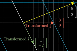
The matrix encodes two column vectors that specify where the two unit vectors (î and ĵ) end up when the vector space is transformed.

Figure 1 shows the two unit vectors (î and ĵ) before the linear transformation and Figure 2 shows the effect of the transformation on those two vectors.

Figure 2: After transformation of the vector space

To find out where any given vector ends up, simply multiply the vector by the matrix.

Consider the yellow arrow in Figure 1 which is represented by the vector

[-1]
[ 2]

Figure 2 shows the effect of the linear transformation on the yellow arrow. In numerical terms, the vector is multiplied by the matrix as follows [3]:

[ 1 3][-1] = -1[ 1] + 2[3] = [-1* 1 + 2*3] = [5]
[-2 0][ 2]     [-2]    [0]   [-1*-2 + 2*0]   [2]

So the place where the vector ends up is -1 times the vector where i-hat ends up plus 2 times the vector where j-hat ends up. That is, the vector started off as a specific linear combination of i-hat and j-hat (-1î + 2ĵ) and it ended up as that same linear combination of where those two unit vectors ended up.

To summarize, a vector is an arrow in space and a matrix is a linear transformation of that space (say, a rotation). So to visualize the arrow in the transformed space, just multiply the vector by the matrix.

Figure 3: Rotate counterclockwise then shear right

It is also possible to apply multiple transformations in succession. In Figure 3, the original vector space is rotated then sheared. The overall effect is another linear transformation, called a composition, that is distinct from the rotation and the shear. The composition (or product) matrix can be calculated by multiplying the rotation matrix by the shear matrix, as follows:

[1 1][0 -1] = [1 -1]
[0 1][1  0]   [1  0]

Note that the first column of the composition matrix shows where i-hat ends up and the second column shows where j-hat ends up. Also note the right-to-left rule [3], so the rotation (blue) occurs first and is then followed by the shear (purple). Order matters, since a shear followed by a rotation would produce a different composition matrix (i.e., the green arrow would end up pointing in a north-west direction). Generally:

[i_x2 j_x2][i_x1 j_x1] = [i_x1i_x2 + i_y1j_x2   j_x1i_x2 + j_y1j_x2]
[i_y2 j_y2][i_y1 j_y1]   [i_x1i_y2 + i_y1j_y2   j_x1i_y2 + j_y1j_y2]

Breaking this down, i and j represent the columns where i-hat and j-hat end up for each matrix. So to calculate where i-hat and j-hat end up in the composition matrix, i and j in the first (blue) matrix each have to be transformed (multiplied) by the second (purple) matrix. So calculating where i-hat ends up first:

[i_x2 j_x2][i_x1] = i_x1[i_x2] + i_y1[j_x2] = [i_x1i_x2 + i_y1j_x2]
[i_y2 j_y2][i_y1]      [i_y2]      [j_y2]   [i_x1i_y2 + i_y1j_y2]

The transformed i-hat vector is the first column of the composition matrix. Similarly calculating where j-hat ends up:

[i_x2 j_x2][j_x1] = j_x1[i_x2] + j_y1[j_x2] = [j_x1i_x2 + j_y1j_x2]
[i_y2 j_y2][j_y1]      [i_y2]      [j_y2]   [j_x1i_y2 + j_y1j_y2]

The transformed j-hat vector is the second column of the composition matrix.

The final effect is that i-hat and j-hat are transformed as indicated by the two columns in the composition matrix. In this way, any number of transformations can be combined in the desired order to produce a new composition matrix.

Consider again the composition of the rotation and shear above. To visualize an arrow in the transformed space, just multiply the vector by the composition matrix. As shown above, the effect is exactly the same as applying the rotation then the shear, except that those two actions are applied in a single action. That is:

[1 1][0 -1][x] = [1 -1][x]
[0 1][1  0][y]   [1  0][y]

It is also possible to represent a transformation between dimensions. A matrix with 3 rows by 2 columns represents a 2D to 3D transformation, whereas a matrix with 2 rows by 3 columns represents a 3D to 2D transformation.

Next up: the determinant of a matrix

--

[1] The figures and examples of the posts in this series are based on the Essence of Linear Algebra series by 3Blue1Brown.

[2] Recall the unit vectors, where î (i-hat) is the arrow of unit length along the X-axis and ĵ (j-hat) is the arrow of unit length along the Y-axis.

Figure 4: Unit vectors

[3] Note that vectors and matrices are multiplied from right to left. The reason for this is that matrices are essentially functions. In function notation, the function M₂(M₁(V)) calculates from inner to outer which, visually, is from right to left. Note also that the order matters because matrix multiplication is non-commutative. That is M₁M₂ != M₂M₁.