Visualizing linear algebra: Introduction

The purpose of this series is to explain the core concepts of linear algebra in a concrete and visual way and is based on the Essence of Linear Algebra series by 3Blue1Brown.

Part 1: Vectors

Part 2: Matrices

Part 3: Determinant

Part 4: Matrix inverse

Part 5: Dot product

Part 6: Cross product

Part 7: Change of basis

Part 8: Eigenvectors

Part 9: Vector spaces

Visualizing linear algebra: Vector spaces

Figure 1: Functions, like vectors, can be added

This is Part 9 in a series on linear algebra [1].

A vector can be represented numerically as a list of numbers or geometrically as an arrow. But is one representation more fundamental than the other or are they both manifestations of something deeper?

A list of numbers seems clear cut and unambiguous when dealing with different dimensions, whether a 2D vector or a 100D vector. Whereas a 4D or higher space can be difficult to describe geometrically. On the other hand, the vector space exists independently of the coordinates that you give it and those coordinates can seem somewhat arbitrary since they depend on your choice of basis vectors. For example, determinants and eigenvectors are inherently spatial (the determinant tells you how much a transformation scales areas and eigenvectors stay on their own span during a transformation) and you can freely change your coordinate system without changing the underlying values of either one.

So if vectors are not fundamentally lists of numbers and their underlying essence is more spatial, then that raises the question of what mathematicians mean when they use a word like space or spatial.

Figure 2: The sum of two functions

It turns out that there is something which is neither an arrow nor a list of numbers but is also a type of vector: functions. In the same way that you can add two vectors together, there is also a sensible notion for adding two functions f and g to get a new function (f + g). That is, the value of the sum function at any given input x is the sum of the values of f(x) + g(x). See Figure 1 which shows two functions and Figure 2 which shows their sum. This is represented as:

(f + g)(x) = f(x) + g(x)

Figure 3: Functions, like vectors, can be scaled

This is similar to adding vectors coordinate by coordinate except that there is, in a sense, infinitely many coordinates to deal with. Similarly, there is a sensible notion for scaling a function by a real number. Just scale all of the outputs by that number For example, as illustrated in Figure 3:

(2f)(x) = 2f(x)

Again, this is analogous to scaling a vector coordinate by coordinate but with infinitely many coordinates.

Now, given that the only thing vectors can really do is get added together or scaled, it seems like we should be able to take the same useful constructs and problem solving techniques of linear algebra (linear transformations, null space, dot products, eigen-everything) that were originally thought about in the context of arrows in space and apply them to functions as well. Such as, for example, the derivative that transforms one function into another function:

^d⁄_dx(3x³ - x) = 9x² - 1

These are sometimes called operators instead of transformations, but the meaning is the same.

Figure 4: Additivity

A transformation is linear if it satisfies two properties, commonly called additivity (see Figure 4) and scaling (see Figure 5).

Additivity means that if you add two vectors, v and w, then apply a transformation to their sum, you get the same result as if you added the transformed versions of v and w. That is:

L(v + w) = L(v) + L(w)

Figure 5: Scaling

The scaling property is that when you scale a vector v by some number, then apply the transformation, you get the same ultimate vector as if you scale the transformed version of v by that same amount. That is:

L(c.v) = c.L(v)

So linear transformations preserve the operations of vector addition and scalar multiplication. These properties also apply to functions such as the derivative. For example:

^d⁄_dx(x³ + x²) = ^d⁄_dx(x³) + ^d⁄_dx(x²)

^d⁄_dx(4x³) = 4 ^d⁄_dx(x³)

Consider the vector space for polynomials. Coordinates are needed for this space which requires choosing a basis. Since polynomials are already written down as the sum of scaled powers of the variable x, it's natural to just choose pure powers of x as the basis function. The first basis function will be the constant function b₀(x)=1, the second basis function will be b₁(x)=x, then b₂(x)=x², then b₃(x)=x³, and so on. The role that these basis functions serve will be similar to the roles of i-hat, j-hat and k-hat in the world of vectors as arrows. For example, the vector [5;3;1;0;0...] (with an infinite tail of zeroes) would be expressed in terms of the basis functions as:

5*1 + 3x + 1x²

Most of the concepts that apply to arrows in space such as linear transformations, the dot product and eigenvectors have direct analogues in the world of functions but with different names such as linear operators, the inner product and eigenfunctions.

Figure 6: Vector spaces

There are lots of vector-like things in math. As long as you're dealing with a set of objects where there's a reasonable notion of scaling and adding, whether that's a set of arrows in space, lists of numbers, functions or whatever else you choose to define, all of the tools developed in linear algebra regarding vectors, linear transformations and so on should be able to apply.

A mathematician need not think about all the different kinds of vector spaces that people might come up with. Instead there are eight axioms that any vector space must satisfy if all the theory and constructs that have been discovered are going to apply. These axioms are not so much fundamental rules of nature as they are an interface between the mathematician who is discovering results and other people who might want to apply those results to new sorts of vector spaces. The axioms serve as a checklist for verifying one's definitions before applying the results of linear algebra. Whereas mathematicians express their results abstractly and only in terms of these axioms. Thus the mathematician's answer to "What are vectors?" is to just ignore the question since the form that vectors take doesn't really matter as long as those rules are followed. Similarly, textbooks and lectures tend to be phrased abstractly to describe the most general case.

And this wraps up the series on visualizing linear algebra!

--

[1] The figures and examples of the posts in this series are based on the Essence of Linear Algebra series by 3Blue1Brown.

Visualizing linear algebra: Eigenvectors

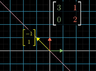
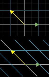
Figure 1: Before transformation

This is Part 8 in a series on linear algebra [1].

A vector that remains on its span [2] when a linear transformation is applied to it is termed an eigenvector of that transformation. The amount that it is scaled is called an eigenvalue.

For example, Figure 1 shows a yellow arrow that will be transformed by the indicated matrix. The purple line is the span of the yellow arrow.

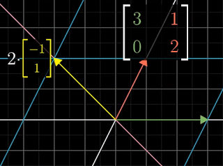
Figure 2: After transformation

Figure 2 shows the yellow arrow after the transformation. Note that the yellow arrow has remained on its span, so it is an eigenvector of the transformation. It has been scaled by a factor of 2, so 2 is the eigenvalue. The eigenvalue is shown as the coefficient of the original vector.

Notice that i-hat is also an eigenvector and its eigenvalue is 3 (i.e., it is scaled by 3). However j-hat has not remained on its span, so it is not an eigenvector of the transformation.

Any vector that lies on the span of either the yellow arrow or the green arrow is an eigenvector and it will also have the eigenvalues 2 and 3 respectively. Any vector, such as the red arrow, that does not lie on either of those spans will be rotated off the line that it spans.

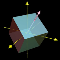
Figure 3: 3D rotation around an axis

Eigenvalues can be negative which means that after the transformation the arrow will point in the opposite direction along its span.

For one example of where finding an eigenvector is useful, consider a 3D dimensional rotation as in Figure 3. If you can find an eigenvector for that transformation, a vector that remains on its own span, then you have found the axis of rotation. For rotations the eigenvalue is always 1 since the length of the vector remains the same.

Note that the columns of a matrix describe the landing spots for the basis vectors. However, as illustrated by the 3D rotation, finding the eigenvectors and eigenvalues describes what the transformation does independent of the particular basis vectors used.

An eigenvector equation can be represented as:

Av = λv

where A is the matrix representing a transformation, v is the eigenvector and λ (lambda) is the corresponding eigenvalue (a number). This expression says that the matrix-vector product (A times v) gives the same result as just scaling the eigenvector v by some value λ. So finding the eigenvectors and their eigenvalues of a matrix A comes down to finding the values of v and λ that make this expression true.

The first step is to convert the right-hand-side of the equation so that it represents a matrix-vector product like the left-hand-side of the equation. This is done by multiplying λ by the identity matrix I, as follows:

Av = (λI)v

Now subtracting the right-hand-side and factoring out v:

Av - λIv = 0
(A - λI)v = 0

We're now looking for a non-zero vector v such that this new matrix times v gives the zero vector. The only way it is possible for the product of a matrix with a non-zero vector to become zero is if the transformation associated with that matrix reduces space to a lower dimension, say, from a plane to a line. In that case, the matrix has a determinant of zero. That is:

det(A - λI) = 0

For example, consider the matrix from Figures 1 and 2:

[3 1]
[0 2]

Now think about subtracting a variable amount λ from each diagonal entry:

[3 1] - λ[1 0] = [3-λ   1]
[0 2]    [0 1]   [  0 2-λ]

The goal is to find any values of λ that will make the determinant of the matrix zero. That is:

det([3-λ   1]) = ad - bc = (3-λ)(2-λ) - 1*0 = (3-λ)(2-λ) = 0
    [  0 2-λ]

Solving this equation, the only possible eigenvalues are λ = 2 and λ = 3.

So when λ equals 2 or 3, the matrix (A - λI) transforms space onto a line. That means there are non-zero vectors v such that (A - λI) times v equals the zero vector. Recall the reason we care about that is because it means Av = λv. That is, the vector v is an eigenvector of A.

To figure out the eigenvectors that have one of these eigenvalues, plug that value of λ into the matrix and then solve for which vectors this diagonally-altered matrix sends to zero. Solving with λ = 2:

[3-2   1][x] = [1 1][x] = x[1] + y[1] = [x+y] = [0]
[  0 2-2][y]   [0 0][y]    [0]    [0]   [  0]   [0]

Since the determinant is zero, there is no unique solution. The solutions are all the vectors on the line described by y = -x which is the diagonal line spanned by [-1;1] or the yellow arrow in Figure 1. Similarly, solving with λ = 3:

[3-3   1][x] = [0  1][x] = x[0] + y[ 1] = [ y] = [0]
[  0 2-3][y]   [0 -1][y]    [0]    [-1]   [-y]   [0]

In this case, the solutions are all the vectors on the line described by y = 0 which is the horizontal line spanned by [1;0] or i-hat in Figure 1.

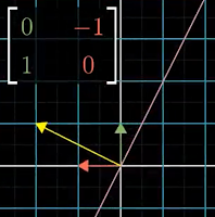
Figure 4: 90° rotation

Not all transformations have eigenvectors. One example is a 2D 90° counterclockwise rotation which rotates all vectors off their spans as shown in Figure 4. Consider computing the eigenvalues of this rotation. Subtract λ from the diagonal elements and look for when the determinant is zero.

det([-λ -1]) = (-λ)(-λ) - -1*1 = 0
    [ 1 -λ]
             = λ² + 1 = 0

∴ λ = i or λ = -i

The only roots of that polynomial are the imaginary numbers i and -i. Assuming we are only looking for real number solutions, there are no eigenvectors for that transformation. However note that eigenvalues that are complex numbers generally correspond to some kind of rotation in the transformation.

Whenever a matrix has zeroes everywhere other than the diagonal, it is called a diagonal matrix. The way to interpret this is that all the basis vectors are eigenvectors with the diagonal entries of the matrix being their eigenvalues. That is, a diagonal matrix simply scales the basis vectors. A diagonal matrix can be represented as a vector times the identity matrix I. For example:

Figure 5: Change of basis

[-1 0] = [1 0][-1]
[ 0 2]   [0 1][ 2]

Therefore, whenever we want to apply a matrix multiplication to a diagonal matrix, it is the same as applying a matrix-vector multiplication, converting an O(N²) operation into O(N).

If a transformation has enough eigenvectors such that you can choose a set that spans the full space, then you can change your coordinate system so that these eigenvectors are your basis vectors. For example, using the eigenvectors for the matrix from Figure 1 as the change of basis matrix (the green and yellow arrows):

[1 -1]^-1[3 1][1 -1] = [3 0]
[0  1]  [0 2][0  1]   [0 2]

This new matrix is guaranteed to be diagonal with its corresponding eigenvalues down that diagonal. The new basis is called an eigenbasis with Figure 5 showing the change of basis. Applying the transformation will scale the new basis vectors by those eigenvalues, that is, the green arrow by 3 and the yellow arrow by 2.

Next up: vector spaces

--

[1] The figures and examples of the posts in this series are based on the Essence of Linear Algebra series by 3Blue1Brown.

[2] A vector that remains on its span either points in the same direction or points in the opposite direction (the negative direction).

Visualizing linear algebra: Change of basis

Figure 1: Alternative basis vectors

This is Part 7 in a series on linear algebra [1].

Any given vector can be understood as the scaling of the unit vectors i-hat and j-hat. These special vectors are the standard basis vectors in a coordinate system.

However it is also possible to use different basis vectors. In Figure 1, the basis vectors b₁ and b₂ point in different directions and have different lengths to i-hat and j-hat.

Figure 2: Alice and Bobs' coordinate systems

Suppose that Alice uses the standard basis vectors i-hat and j-hat while Bob uses the alternative basis vectors b₁ and b₂. While Alice and Bob are looking at the same vectors in space, they can be considered to be using different languages to refer to them.

In Figure 2, Alice would describe b₁ with the vector coordinates [2;1] and b₂ with the vector coordinates [-1;1].[2] Whereas from Bob's perspective, b₁ and b₂ have coordinates [1;0] and [0;1]. They are what define the meaning of the coordinates [1;0] and [0;1] in his system. To reiterate, both Alice and Bob are looking at the same vectors in space, but they use different words and numbers to describe them.

Figure 3: Vector [-1;2] in Bob's system

To translate between Alice and Bobs' coordinate systems, consider Figure 3. Suppose Bob describes a vector with coordinates [-1;2] in his system. That is, b₁ is scaled by -1 and b₂ is scaled by 2 as represented by the yellow arrow. From Alice's perspective, the coordinates for b₁ and b₂ in her system can be similarly scaled to describe the vector in her system. That is:

-1[2] + 2[-1] = [-4]

  [1]    [ 1]   [ 1]

Note that this is just matrix-vector multiplication with a matrix whose column vectors represent Bob's basis vectors in Alice's language. That is:

[2 -1][-1] = -1[2] + 2[-1] = [-4]

[1  1][ 2]     [1]    [ 1]   [ 1]

In effect, a matrix whose column vectors represent Bob's basis vectors can be thought of as a transformation that moves Alice's basis vectors, i-hat and j-hat, to Bob's basis vectors, b₁ and b₂. So the vector [-1;2] is a certain linear combination of Alice's basis vectors (-1î + 2ĵ ). The resulting vector after the transformation will be that same linear combination but of the new basis vectors (-1b₁ + 2b₂). This transformation, in essence, enables Alice to describe vectors in Bob's language.

It is similarly possible for Bob to describe vectors in Alice's language. This requires taking the inverse of the matrix which corresponds to playing the transformation backwards. The inverse of the matrix is:

[2 -1]^-1 = [ 1/3 1/3]

[1  1]     [-1/3 2/3]

Let's go in the other direction, taking the vector that Alice describes in her language above as [-4;1] and describe it in Bob's language:

[ 1/3 1/3][-4] = -4[ 1/3] + 1[1/3] = [-1]

[-1/3 2/3][ 1]     [-1/3]    [2/3]   [ 2]

The result is [-1;2] in Bob's language which is verified by the yellow arrow in Figure 3.

That is how to translate the descriptions of individual vectors back and forth between coordinate systems. The matrix whose columns represent Bob's basis vectors but written in Alice's coordinates translates vectors from Bob's language into Alice's. And the inverse matrix does the opposite.

Linear transformations involving matrices can also be described in different coordinate systems. For example, a 90° counterclockwise rotation can be described in Alice's system as:

[0 -1]
[1  0]

That is, i-hat ends up at coordinates [0;1] and j-hat ends up at coordinates [-1;0]. To translate this into Bob's system, first consider a vector in Bob's language, say, the vector [-1;2] from above. That vector needs to be translated to Alice's language using the change of basis matrix, then the rotation applied in Alice's language, then translated back to Bob's language using the inverse change of basis matrix. This can be represented, from right-to-left, as:

[2 -1]^-1[0 -1][2 -1][-1]
[1  1]  [1  0][1  1][ 2]

This transformation sequence will work for any vector in Bob's language. The product of the three matrices is:

[2 -1]^-1[0 -1][2 -1] = [1/3 -2/3]

[1  1]  [1  0][1  1]   [5/3 -1/3]

If Bob applies this composition matrix to a vector in his system, it will return the rotated version of that vector expressed in his coordinate system. For example:

[1/3 -2/3][1] = [-1]

[5/3 -1/3][2]   [ 1]

With an expression like A^-1MA , the middle matrix represents a transformation M as one person sees it, the outer matrices indicate the shift in perspective, while the full matrix product represents a transformation M as someone else sees it.

Next up: eigenvectors

--

[1] The figures and examples of the posts in this series are based on the Essence of Linear Algebra series by 3Blue1Brown.

[2] The notation [x;y] using a semicolon indicates a column vector.

Visualizing linear algebra: Cross product

Figure 1: The red arrow is the cross product of
the purple and orange arrows

This is Part 6 in a series on linear algebra [1].

As described in the post on matrices, a 2x2 matrix encodes two column vectors that show where the two unit vectors (i-hat and j-hat) end up when the 2D vector space is transformed. The post on the determinant shows how the unit square defined by those unit vectors is transformed into a parallelogram. The determinant is a measure of the area of the parallelogram which can be negative if i-hat ends up on the left of j-hat, thus indicating the area was flipped, or zero if i-hat and j-hat end up on the same line.

The 3D cross product of two vectors is a third vector that is perpendicular to both and has a length that is their determinant (i.e., the directional area of the parallelogram defined by those vectors) as illustrated in Figure 1. [2]

Figure 2: Solve for vector p

Figure 2 shows the equation for computing a vector p that is the cross product of vectors v and w.

Algebraically, the equation asks what is the vector p such that the dot product of p and a vector [x;y;z] equals the determinant of a 3x3 matrix with column vectors [x;y;z], v and w?

Geometrically, the equation asks what is the vector p such that projecting vector [x;y;z] onto its number line and scaling by the length of p will equal the signed volume of a parallelepiped defined by the vectors [x;y;z], v and w?

The equation can be reorganized as:

p₁.x + p₂.y + p₃.z = x(v₂.w₃ - v₃.w₂) +

                     y(v₃.w₁ - v₁.w₃) +
                     z(v₁.w₂ - v₂.w₁)

The constants on the right hand side are particular combinations of the coordinates of v and w which will be the coordinates of p and thus the cross product of v and w:

            [v₂.w₃ - v₃.w₂]

p = v x w = [v₃.w₁ - v₁.w₃]
            [v₁.w₂ - v₂.w₁]

Figure 3 illustrates that the way the linear transformation works on a given vector [x;y;z] (the white arrow) is to project that vector onto a line p (the red arrow) that's perpendicular to both v and w and then to scale that projection by the area of the parallelogram spanned by v and w. This is the same thing as taking a dot product between [x;y;z] and a vector that's perpendicular to v and w with a length equal to the area of that parallelogram.

Next up: change of basis

--

[1] The figures and examples of the posts in this series are based on the Essence of Linear Algebra series by 3Blue1Brown.

[2] The cross product is used in a 3D vector space where the third vector is computed from the first two. If used in 2D space, it would return a vector that was perpendicular to that 2D space.

Visualizing linear algebra: Dot product

Figure 1: Column vector as an arrow

This is Part 5 in a series on linear algebra [1].

Figure 1 shows a vector that is represented geometrically as a yellow arrow and numerically as a column. It scales the unit vectors i-hat and j-hat by 2 and 4 respectively. That is:

v = 2î + 4ĵ

Now suppose the column is transposed to a row, as follows:

[2]^T = [2 4]
[4]

This row is a 2x1 matrix that represents the transformation of a 2D vector space to a 1D vector space, that is, a number line. The number line is the span of the yellow arrow (i.e., it extends along the yellow arrow in both directions).

Figure 2: Row vector as a transformation matrix

The effect of this transformation on the unit vectors is shown in Figure 2 where i-hat is scaled by 2 and j-hat is scaled by 4. The length of the yellow arrow, per Pythagoras' Theorem, is √(2² + 4²) =  √20, or about 4.47.

For any given input vector, the position on the number line where the input vector ends up will be the vector's X coordinate scaled by 2 plus the vector's Y coordinate scaled by 4.

Figure 3: Calculating the dot product

For example, the purple arrow in Figure 3 is transformed to a 1D vector, or scalar, on the number line as follows:

[2 4][2] = 2[2] + 1[4] = 8
     [1]

Geometrically, this is equivalent to projecting the purple arrow onto the span of the yellow arrow (at position 8/√20, or 1.79) and scaling by the length of the yellow arrow (√20, or 4.47). The small right-angled triangle in Figure 3 shows the projection.

In the symmetrical example where the column for the purple arrow is transposed to a row (representing a transformation to the number line that is the span of the purple arrow), the yellow arrow is transformed as follows:

[2 1][2] = 2[2] + 4[1] = 8
     [4]

The scalar result is the same as for the first example - the vector order doesn't matter. However geometrically, it is equivalent to projecting the yellow arrow onto the span of the purple arrow (at position 8/√5, or 3.58) and scaling by the the length of the purple arrow (√(2² + 1²) =  √5, or 2.24). The large right-angled triangle in Figure 3 shows the projection.

More generally, this operation is the dot product (or scalar product) of two vectors and for 2D vectors is defined [2] as:

a.b = a_xb_x + a_yb_y

When the arrows are pointing in the same general direction the dot product is positive, when pointing in the opposite direction the dot product is negative, and when the arrows are orthogonal the dot product is zero.

Figure 4: Dot product = transform

Numerically the dot product multiplies two vectors, taking direction into account [3].

Geometrically, one vector encodes a linear transformation that projects space onto a number line and scales the projection by the length of the vector.

Next up: the cross product

--

[1] The figures and examples of the posts in this series are based on the Essence of Linear Algebra series by 3Blue1Brown.

[2] The dot product is also defined as

a.b = ∥a∥∥b∥cos(θ)

where ∥v∥ denotes the magnitude of vector v. This can also be interpreted as projecting one of the vectors onto the other vector (via the cosine) and scaling by the other vector.

[3] The numerical summary comes from Better Explained which also offers further analogies.