Visualizing quantum computations

Figure 1: Quantum parallelism

You are presented with an opaque box that has two buttons labelled A and B. Each button is programmed to glow either red or green when pressed. Can you determine, without investigating inside the box, whether the two buttons are programmed to show the same color or different colors?

The answer, of course, can be determined by pressing each button to see what it does. And it is necessary to press both buttons - pressing just one button won't convey enough information to determine the answer.

Figure 2: Black box function

This scenario can be represented in an algorithm using two binary digits (bits) to represent the color that glows when each respective button is pressed. Analogous to the opaque box, the function that retrieves information about the bits is a black box (see Figure 2) where our focus (for now) is on the inputs and outputs. The algorithm is outlined in the following code fragment.

 1: // constant bit definitions
 2: bitButtonIndex { A = 0, B = 1 }
 3: bitColorIndex { red = 0, green = 1 }
 4:
 5: // black box function declaration
 6: f(input bitButtonIndex) output bitColorIndex;
 7:
 8: bitColorForButtonA = f(A);
 9: bitColorForButtonB = f(B);
10: if (bitColorForButtonA == bitColorForButtonB) then
11:   bitButtonsShowTheSameColor = yes;
12: else
13:   bitButtonsShowTheSameColor = no;

The important thing to note about the above is that the black box function needs to be called twice to determine whether the buttons show the same color.

This same scenario can also be represented on a quantum computer. However in this case the black box function accepts a qubit as input containing the button information and returns a qubit as output containing the color information. The quantum algorithm is outlined in the following code fragment.

 1: // quantum black box function declaration
 2: Uf(input/output qubitX, qubitY); // |x,y> -> |x,y⊕f(x)>
 3:

 4: // variable declarations

 5: qubit x;  // x holds button or (later) color information
 6: qubit y;  // y facilitates use of the black box function
 7:
 8: x = |0>;  // prepare x in a known state

 9: H(x);     // transform x to |+>, i.e., 1/√2(|0> + |1>)

10:
11: y = |0>;  // prepare y in a known state

12: X(y);     // flip state of y to |1>

13: H(y);     // transform y to |->, i.e., 1/√2(|0> - |1>)

14:

15: Uf(x, y); // transform x to |+> or |->

16. H(x);     // transform x from |+> to |0> or from |-> to |1>

17:

18: bitMeasurementResult = M(x); // measure the value of x
19: if (bitMeasurementResult  == 0) then
20:   bitButtonsShowTheSameColor = yes;
21: else
22:   bitButtonsShowTheSameColor = no;

Note that the quantum black box function only needs to be called once to determine whether the buttons show the same color. While the classical function only processes a single specific button at one time, the quantum function can process both button indexes simultaneously. This is represented by the (superposed) state of x as 1/√2(0> + |1>) prior to the call to Uf, where 0 and 1 have the same meaning as per the classical algorithm (i.e., as button indexes for A and B respectively).[1]

Before going into the details of the above code, this algorithm (called Deutsch's Algorithm) is probably the simplest example demonstrating the parallelism of quantum computing - the ability to evaluate all possible inputs to a function simultaneously. Qubits can also be combined to exponentially increase the parallelism. For example, Figure 1 shows a single four-bit input that is processed by a classical computer to produce a single four-bit output. Compare that to the four-qubit input that allows up to 2⁴, or 16, superposed values to be input and then simultaneously processed by a quantum computer to produce 16 superposed values as output.

But there is a major problem! If the qubit returned by the quantum function is in superposition and it is measured, then the superposed state randomly collapses to just one of the two basis states (|0> or |1>) - a single bit of information! So the quantum function needs to encode the answer to our final question such that it can be successfully extracted by a measurement. While quantum computing promises exponential speedup and memory efficiencies, the challenge is to construct algorithms that amplify the right answer and cancel out wrong answers such that the right answer will be measured with high probability.

In fact, this is what the above algorithm is able to do. Note that unlike the classical algorithm, the black box function does not return the colors associated with the specific buttons. Instead, the function returns a result that represents the relative difference in the button colors (if any), whatever those colors happen to be.

Figure 3: Quantum circuit for Deutsch's Algorithm

Now let's turn to the details of the quantum algorithm. The circuit for this algorithm is illustrated in Figure 3. The circuit shows qubit x on the top wire and qubit y on the bottom wire as they are transformed over time (from left-to-right). In quantum mechanics, the functions (or logic gates) are unitary which means, among other things, that they are reversible. Note that the black box function (also termed a quantum oracle) specifies y⊕f(x) as an output. The ⊕ symbol represents an exclusive or (xor) operation.

Per line 9, input x is in state 1/√2(|0> + |1>), representing a superposition of pressing button A and pressing button B. Recall that 0 represents button A and 1 represents button B. If button A glows green, a 180° phase change is applied to state |0>. Similarly, if button B glows green, a 180° phase change is applied to state |1>. This can be expressed by the following formula (derived in [2]) where f is the original classical black box function:

1/√2((-1)^f(0)|0> + (-1)^f(1)|1>)

This reduces to one of the four output states in the following table which can then be changed back to the computational basis state with a Hadamard transform. Note that the measurement ignores the global phase (i.e., the leading minus signs).

Btn A   Btn B  |                                       Same
 f(0)    f(1)  |     Output x      Hadamard   Measure  color?
---------------+---------------------------------------------
red:0   red:0  |   1/√2(|0> + |1>)    |0>        0      yes
grn:1   grn:1  |  -1/√2(|0> + |1>)   -|0>        0      yes
red:0   grn:1  |   1/√2(|0> - |1>)    |1>        1      no
grn:1   red:0  |  -1/√2(|0> - |1>)   -|1>        1      no

Note that the phase change formula and the color results are a mathematical representation of what is occurring within the quantum black box function. While we can measure the output qubit, we cannot access the specific button color information (which is encoded in the phase of the states). Nonetheless the information we can access is sufficient to determine whether the colors are the same.

Figure 4: MZI with a glass sample representing the
color green when button A is pressed

Our original scenario can be modified to utilize quantum parallelism by using a Mach-Zehnder interferometer as our quantum black box. When the paths of the MZI are equal in length (and no samples are present), a photon entering the MZI (and travelling in a superposition of both paths) will always end up at detector 1. To model our scenario, the upper path will represent the pressing of button A while the lower path will represent the pressing of button B. A glass sample placed on either or both of the paths will represent the color green while its absence will represent the color red. The thickness of the glass sample is such that it will change the phase of the photon passing through it by 180°.

The effect of placing a sample on just one of the paths is that the interference at the final beam splitter will result in the photon always ending up at detector 2. Placing a sample on both paths means the photon will accumulate identical phase changes on each path which cancel out. So the effect is that the photon will always end up at detector 1 just as it would when there are no samples present. The glass samples thus implement the exclusive or (xor) operation in our quantum black box. While we are not able to determine the specific colors of the buttons (without investigating inside the black box), we can determine whether the colors are the same or not by observing which detector the photon arrives at.

References:

• Blog post on visualizing qubits
• Blog post on modeling quantum interference
• Quantum Algorithm with an example - Jonathan Hui
• Lecture on the Deutsch Algorithm - Scott Aaronson
• Q#: A Quantum Programming Language by Microsoft
• Simulating a Quantum Computer with a Mach-Zehnder Interferometer - Frank Rioux

"Suppose you are asked if two pieces of glass are the same thickness. The conventional thing to do is to measure the thickness of each piece of glass and then compare the results. As David Deutsch pointed out this is overkill. You were asked only if they were the same thickness, but you made two measurements to answer that question, when in fact it can be done with one." - Frank Rioux

--

[1] The coefficient of 1/√2 is the probability amplitude which, when squared, gives the probability of measuring the associated state. In this case, there is a 1/2 probability of measuring 0 and a 1/2 probability of measuring 1.

[2] The quantum black box function maps |x,y> to |x,y⊕f(x)) where ⊕ symbolizes xor. The input qubits to the function are:

|x> = 1/√2(|0> + |1>)
|y> = 1/√2(|0> - |1>)

Combining the two inputs (where ⊗ symbolizes the tensor product):

|x,y> = 1/√2(|0> + |1>) ⊗ 1/√2(|0> - |1>)
      = 1/2(|0> + |1>)(|0> - |1>)
      = 1/2(|0>(|0> - |1>) +
            |1>(|0> - |1>))

Substituting y⊕f(x) for y:

|x,y⊕f(x)> = 1/2(|0>(|0⊕f(0)> - |1⊕f(0)>) +
                   |1>(|0⊕f(1)> - |1⊕f(1)>))

When f(x) = 0 (indicating red), the state remains unchanged. When f(x) = 1 (indicating green), the sign is flipped. This effect on the phase can be represented as (-1)^f(x) giving (-1)⁰ = 1 and (-1)¹ = -1 respectively. Continuing:

            = 1/2(|0>((-1)^f(0)|0> - (-1)^f(0)|1>) +
                  |1>((-1)^f(1)|0> - (-1)^f(1)|1>))
            = 1/2((-1)^f(0)|0>(|0> - |1>) +
                  (-1)^f(1)|1>(|0> - |1>))
            = 1/2((-1)^f(0)|0> + (-1)^f(1)|1>)(|0> - |1>)
            = 1/√2((-1)^f(0)|0> + (-1)^f(1)|1>) ⊗ 1/√2(|0> - |1>)

So the separate output qubits of the quantum black box function are:

|x> = 1/√2((-1)^f(0)|0> + (-1)^f(1)|1>)
|y> = 1/√2(|0> - |1>)

Note: The reversible xor operation is implemented using a CNOT gate. When applied in the computational basis { |0>,|1> }, x is the control qubit and y is the target qubit. However when applied in the Hadamard basis { |+>,|-> } as above, y becomes the control qubit and x becomes the target qubit, as explained here.

Visualizing qubits

Figure 1: Classical and quantum bits

In classical computing, the basic unit of information is the bit (or binary digit). As illustrated in Figure 1, a bit can be in one of two states as represented by the values 0 and 1. [1] This can be physically implemented in various ways such as by two distinct voltage levels in a circuit or by a switch. As the basic unit of information, the bit abstracts over the physical implementation, allowing the programmer to work with that abstraction rather than the details of the underlying hardware and physics.

In quantum computing, the basic unit of information is the qubit (or quantum bit). When a qubit is measured (a read operation), it exhibits the same characteristics as a classical bit. That is, a value of 0 or 1 is returned. This is illustrated in Figure 1 by the points at the north and south poles of the sphere. However, as suggested by the sphere visualization, the state of a qubit is very different to the state of a classical bit. As well as being in a state of 0 or 1, a qubit can also be transformed into a superposition of those two states which is represented by a point elsewhere on the surface of the sphere.[2]

Figure 2: Qubit vector space
(imaginary dimensions omitted)

But set aside the sphere visualization for the moment. In quantum computing, the state of a qubit is represented by a vector in a vector space. The vector space is two dimensional with the two standard basis vectors representing the values of 0 and 1 (see Figure 2, where the basis vectors are denoted in ket notation as |0> and |1>).  The state of the qubit can be one of the two basis vectors or a linear combination of both and is denoted as |ψ> (psi). The length of the vector is always 1 (i.e., terminating on the unit circle). Finally, the vector space is complex rather than real which means the coefficients α and β of the basis states are complex numbers. In ket notation, this would be:

|ψ> = α|0> + β|1>

Note that each complex number has two degrees of freedom (i.e., a complex number has a real component and an imaginary component) for a total of four degrees of freedom. The 2D Cartesian plane in Figure 2 shows only the real components of α and β.

Figure 3: The Bloch sphere

However it is possible to do better. Note that the length of |ψ> must always be 1. That is, |α|² + |β|² = 1. This removes one degree of freedom. In addition, only the relative difference between the complex phases of the states has observable consequences. For example, if one state has a phase of π/2 and the other a phase of 3π/2, the relative difference around the complex plane is π. So this removes another degree of freedom leaving just two degrees of freedom. It is now possible to visualize the state of the qubit on the surface of a sphere (called the Bloch sphere). In Figure 3, |ψ> is represented by a vector (orange) radiating from the center of the sphere to a point on the surface. The latitude is designated by the polar angle from the Z-axis (θ or theta) and the longitude is designated by the azimuthal angle from the X-axis (φ or phi).

In the Bloch sphere representation, the basis states |0> and |1> are shown at the north and south poles. When a measurement is performed on the qubit, the vector |ψ> collapses to one of the two basis states and a value of 0 or 1 is measured. The closer the point is to one of the poles, the more likely that a measurement of the qubit will collapse the state to that pole. More precisely, the probability that a particular value is measured is the square of the coefficient for that state.[3] The state coefficients can be calculated from the angles as follows:

α = cos(θ/2)
β = e^iφ sin(θ/2)

where e^iφ is the physically significant relative phase. In effect, the XY plane is the complex plane that locates the phase while the position along the Z-axis indicates the probability of measuring a particular state.[4]

The vector |ψ> is moved to new locations on the sphere via rotations around the X, Y and Z axes. To rotate around an axis, the following Pauli matrices are used:[5]

X = [0 1]   Y = [0 -i]   Z = [1  0]
    [1 0]       [i  0]       [0 -1]

Other rotations include the Hadamard matrix and the Phase shift matrix:

H = 1/√2[1  1]   S = [1 0]
        [1 -1]       [0 i]

These matrices transform between the different Pauli-basis states, i.e., H: {|0>,|1>} to {|+>,|->} and S: {|+>,|->} to {|+i>,|-i>}. [6] As an example, suppose the the qubit is prepared in state |0>. Applying the Hadamard matrix gives:

|ψ> = 1/√2[1  1][1] = 1/√2[1] = 1/√2(|0> + |1>)
          [1 -1][0]       [1]

This represents a superposition where |ψ> is located at the point denoted by X on the sphere (the |+> state). The square of the amplitude for each state is 0.5 so, if a measurement is taken, there is a 50% probability of measuring 0 or 1. Applying the Phase shift matrix gives:

|ψ> = [1 0][1/√2] = 1/√2[1] = 1/√2(|0> + i|1>)
      [0 i][1/√2]       [i]

This represents a superposition where |ψ> is located at the point denoted by Y on the sphere (the |+i> state).

To visualize the qubit states for different angles, try the Bloch sphere simulator.

To summarize so far, a qubit can contain a seemingly unlimited amount of information since the point on the Bloch sphere representing the qubit state can be extremely fine-grained. However the information extracted by a measurement is always 0 or 1 (with the probability depending on the latitude of the point on the sphere).

Now consider the combination of multiple qubits. While a 2-bit system can hold only one value between 0 and 3 (2² - 1) at one time, a 2-qubit system can hold all 4 values in superposition at the same time. This provides an exponentially larger computation space with computations able to be performed on all the values in parallel. For a sense of what this means, consider that a 300-qubit system in superposition provides 2³⁰⁰ simultaneous values - more than the number of atoms in the observable universe.

For a 2-qubit system, a superposition is produced by preparing both qubits in the |0> state and then applying a Hadamard gate, as follows:

|ψ> = H|00>
    = 1/√2(|0> + |1>) ⊗ 1/√2(|0> + |1>)
    = 1/2(|00> + |01> + |10> + |11>)

This is called a separable (or unentangled) state because the composite system is separable into two subsystems (i.e., one for each qubit) as the second line indicates.[7] In this case, if one of the qubits were measured then the other qubit value could still be either 0 or 1 since the two qubits are independent.

Figure 4: Preparing a Bell state

Alternatively, a maximally entangled state, called a Bell state, can be produced by preparing both qubits in the |0> state and then applying a Hadamard gate to the first qubit (and an Identity gate to the second qubit) and a CNOT gate [8] to both qubits, as follows:

|ψ> = CNOT (H⊗I)|00>
    = CNOT 1/√2(|0> + |1>)|0>
    = 1/√2(|00> + |11>)

The two qubits are no longer independent of each other. In this case, if one of the qubits were measured, then the other qubit would have the same value when measured.

To solve a problem on a quantum computer, interference between states needs to be exploited to amplify signals leading to the right answer and cancel signals leading to the wrong answer. This requires designing algorithms that exploit specific features of the problem such that when the system is measured, the desired answer is obtained.

--

[1] Or a similar two-state representation such as true and false or on and off.

[2] As with a classical bit, a qubit can also be physically implemented in various ways, such as by the ground and excited states of a particle or by the spin-up and spin-down states of a particle.

[3] This is the Born rule.

[4] The states α|0> + β|1>, α|0> − β|1> and α|0> + iβ|1> all have the same measurement probabilities in the standard basis. However they are distinct states due to their phase differences and therefore behave differently in terms of how they evolve. Also, the probabilities can differ when measured in a different basis.

[5] Recall that

|ψ> = cos(θ/2)|0> + e^iφ sin(θ/2)|1>

X = [0 1]   Y = [0 -i]   Z = [1  0]
    [1 0]       [i  0]       [0 -1]

The Pauli matrices X, Y and Z give rise to the rotation operators about the x, y and z axes of the Bloch sphere:

R_x(θ) = e^-iθX/2 = [ cos(θ/2)     -i.sin(θ/2) ]
                  [ -i.sin(θ/2)  cos(θ/2)    ]
R_y(θ) = e^-iθY/2 = [ cos(θ/2)     -sin(θ/2)   ]
                  [ sin(θ/2)     cos(θ/2)    ]
R_z(θ) = e^-iθZ/2 = [ e^-iθ/2        0            ]
                  [ 0             e^iθ/2         ]

[6] The basis states corresponding to each axis (illustrated in Figure 5) are:

X: 1/√2(|0> + |1>),1/√2(|0> - |1>) or |+>,|-> (the diagonal or plus-minus basis)

Y: 1/√2(|0> + i|1>),1/√2(|0> - i|1>) or |+i>,|-i> (the circular or right-left basis)

Z: |0>,|1> (the up-down, standard or computational basis)

Figure 5: Basis states for each axis

[7] V ⊗ W represents the product of two vector spaces, itself a vector space.

[8] The CNOT gate flips the second qubit (the target qubit) if and only if the first qubit (the control qubit) is |1>.

Visualizing linear algebra: Introduction

The purpose of this series is to explain the core concepts of linear algebra in a concrete and visual way and is based on the Essence of Linear Algebra series by 3Blue1Brown.

Part 1: Vectors

Part 2: Matrices

Part 3: Determinant

Part 4: Matrix inverse

Part 5: Dot product

Part 6: Cross product

Part 7: Change of basis

Part 8: Eigenvectors

Part 9: Vector spaces

Visualizing linear algebra: Vector spaces

Figure 1: Functions, like vectors, can be added

This is Part 9 in a series on linear algebra [1].

A vector can be represented numerically as a list of numbers or geometrically as an arrow. But is one representation more fundamental than the other or are they both manifestations of something deeper?

A list of numbers seems clear cut and unambiguous when dealing with different dimensions, whether a 2D vector or a 100D vector. Whereas a 4D or higher space can be difficult to describe geometrically. On the other hand, the vector space exists independently of the coordinates that you give it and those coordinates can seem somewhat arbitrary since they depend on your choice of basis vectors. For example, determinants and eigenvectors are inherently spatial (the determinant tells you how much a transformation scales areas and eigenvectors stay on their own span during a transformation) and you can freely change your coordinate system without changing the underlying values of either one.

So if vectors are not fundamentally lists of numbers and their underlying essence is more spatial, then that raises the question of what mathematicians mean when they use a word like space or spatial.

Figure 2: The sum of two functions

It turns out that there is something which is neither an arrow nor a list of numbers but is also a type of vector: functions. In the same way that you can add two vectors together, there is also a sensible notion for adding two functions f and g to get a new function (f + g). That is, the value of the sum function at any given input x is the sum of the values of f(x) + g(x). See Figure 1 which shows two functions and Figure 2 which shows their sum. This is represented as:

(f + g)(x) = f(x) + g(x)

Figure 3: Functions, like vectors, can be scaled

This is similar to adding vectors coordinate by coordinate except that there is, in a sense, infinitely many coordinates to deal with. Similarly, there is a sensible notion for scaling a function by a real number. Just scale all of the outputs by that number For example, as illustrated in Figure 3:

(2f)(x) = 2f(x)

Again, this is analogous to scaling a vector coordinate by coordinate but with infinitely many coordinates.

Now, given that the only thing vectors can really do is get added together or scaled, it seems like we should be able to take the same useful constructs and problem solving techniques of linear algebra (linear transformations, null space, dot products, eigen-everything) that were originally thought about in the context of arrows in space and apply them to functions as well. Such as, for example, the derivative that transforms one function into another function:

^d⁄_dx(3x³ - x) = 9x² - 1

These are sometimes called operators instead of transformations, but the meaning is the same.

Figure 4: Additivity

A transformation is linear if it satisfies two properties, commonly called additivity (see Figure 4) and scaling (see Figure 5).

Additivity means that if you add two vectors, v and w, then apply a transformation to their sum, you get the same result as if you added the transformed versions of v and w. That is:

L(v + w) = L(v) + L(w)

Figure 5: Scaling

The scaling property is that when you scale a vector v by some number, then apply the transformation, you get the same ultimate vector as if you scale the transformed version of v by that same amount. That is:

L(c.v) = c.L(v)

So linear transformations preserve the operations of vector addition and scalar multiplication. These properties also apply to functions such as the derivative. For example:

^d⁄_dx(x³ + x²) = ^d⁄_dx(x³) + ^d⁄_dx(x²)

^d⁄_dx(4x³) = 4 ^d⁄_dx(x³)

Consider the vector space for polynomials. Coordinates are needed for this space which requires choosing a basis. Since polynomials are already written down as the sum of scaled powers of the variable x, it's natural to just choose pure powers of x as the basis function. The first basis function will be the constant function b₀(x)=1, the second basis function will be b₁(x)=x, then b₂(x)=x², then b₃(x)=x³, and so on. The role that these basis functions serve will be similar to the roles of i-hat, j-hat and k-hat in the world of vectors as arrows. For example, the vector [5;3;1;0;0...] (with an infinite tail of zeroes) would be expressed in terms of the basis functions as:

5*1 + 3x + 1x²

Most of the concepts that apply to arrows in space such as linear transformations, the dot product and eigenvectors have direct analogues in the world of functions but with different names such as linear operators, the inner product and eigenfunctions.

Figure 6: Vector spaces

There are lots of vector-like things in math. As long as you're dealing with a set of objects where there's a reasonable notion of scaling and adding, whether that's a set of arrows in space, lists of numbers, functions or whatever else you choose to define, all of the tools developed in linear algebra regarding vectors, linear transformations and so on should be able to apply.

A mathematician need not think about all the different kinds of vector spaces that people might come up with. Instead there are eight axioms that any vector space must satisfy if all the theory and constructs that have been discovered are going to apply. These axioms are not so much fundamental rules of nature as they are an interface between the mathematician who is discovering results and other people who might want to apply those results to new sorts of vector spaces. The axioms serve as a checklist for verifying one's definitions before applying the results of linear algebra. Whereas mathematicians express their results abstractly and only in terms of these axioms. Thus the mathematician's answer to "What are vectors?" is to just ignore the question since the form that vectors take doesn't really matter as long as those rules are followed. Similarly, textbooks and lectures tend to be phrased abstractly to describe the most general case.

And this wraps up the series on visualizing linear algebra!

--

[1] The figures and examples of the posts in this series are based on the Essence of Linear Algebra series by 3Blue1Brown.

Visualizing linear algebra: Eigenvectors

Figure 1: Before transformation

This is Part 8 in a series on linear algebra [1].

A vector that remains on its span [2] when a linear transformation is applied to it is termed an eigenvector of that transformation. The amount that it is scaled is called an eigenvalue.

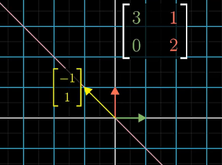
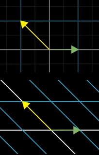
For example, Figure 1 shows a yellow arrow that will be transformed by the indicated matrix. The purple line is the span of the yellow arrow.

Figure 2: After transformation

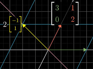
Figure 2 shows the yellow arrow after the transformation. Note that the yellow arrow has remained on its span, so it is an eigenvector of the transformation. It has been scaled by a factor of 2, so 2 is the eigenvalue. The eigenvalue is shown as the coefficient of the original vector.

Notice that i-hat is also an eigenvector and its eigenvalue is 3 (i.e., it is scaled by 3). However j-hat has not remained on its span, so it is not an eigenvector of the transformation.

Any vector that lies on the span of either the yellow arrow or the green arrow is an eigenvector and it will also have the eigenvalues 2 and 3 respectively. Any vector, such as the red arrow, that does not lie on either of those spans will be rotated off the line that it spans.

Figure 3: 3D rotation around an axis

Eigenvalues can be negative which means that after the transformation the arrow will point in the opposite direction along its span.

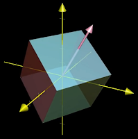
For one example of where finding an eigenvector is useful, consider a 3D dimensional rotation as in Figure 3. If you can find an eigenvector for that transformation, a vector that remains on its own span, then you have found the axis of rotation. For rotations the eigenvalue is always 1 since the length of the vector remains the same.

Note that the columns of a matrix describe the landing spots for the basis vectors. However, as illustrated by the 3D rotation, finding the eigenvectors and eigenvalues describes what the transformation does independent of the particular basis vectors used.

An eigenvector equation can be represented as:

Av = λv

where A is the matrix representing a transformation, v is the eigenvector and λ (lambda) is the corresponding eigenvalue (a number). This expression says that the matrix-vector product (A times v) gives the same result as just scaling the eigenvector v by some value λ. So finding the eigenvectors and their eigenvalues of a matrix A comes down to finding the values of v and λ that make this expression true.

The first step is to convert the right-hand-side of the equation so that it represents a matrix-vector product like the left-hand-side of the equation. This is done by multiplying λ by the identity matrix I, as follows:

Av = (λI)v

Now subtracting the right-hand-side and factoring out v:

Av - λIv = 0
(A - λI)v = 0

We're now looking for a non-zero vector v such that this new matrix times v gives the zero vector. The only way it is possible for the product of a matrix with a non-zero vector to become zero is if the transformation associated with that matrix reduces space to a lower dimension, say, from a plane to a line. In that case, the matrix has a determinant of zero. That is:

det(A - λI) = 0

For example, consider the matrix from Figures 1 and 2:

[3 1]
[0 2]

Now think about subtracting a variable amount λ from each diagonal entry:

[3 1] - λ[1 0] = [3-λ   1]
[0 2]    [0 1]   [  0 2-λ]

The goal is to find any values of λ that will make the determinant of the matrix zero. That is:

det([3-λ   1]) = ad - bc = (3-λ)(2-λ) - 1*0 = (3-λ)(2-λ) = 0
    [  0 2-λ]

Solving this equation, the only possible eigenvalues are λ = 2 and λ = 3.

So when λ equals 2 or 3, the matrix (A - λI) transforms space onto a line. That means there are non-zero vectors v such that (A - λI) times v equals the zero vector. Recall the reason we care about that is because it means Av = λv. That is, the vector v is an eigenvector of A.

To figure out the eigenvectors that have one of these eigenvalues, plug that value of λ into the matrix and then solve for which vectors this diagonally-altered matrix sends to zero. Solving with λ = 2:

[3-2   1][x] = [1 1][x] = x[1] + y[1] = [x+y] = [0]
[  0 2-2][y]   [0 0][y]    [0]    [0]   [  0]   [0]

Since the determinant is zero, there is no unique solution. The solutions are all the vectors on the line described by y = -x which is the diagonal line spanned by [-1;1] or the yellow arrow in Figure 1. Similarly, solving with λ = 3:

[3-3   1][x] = [0  1][x] = x[0] + y[ 1] = [ y] = [0]
[  0 2-3][y]   [0 -1][y]    [0]    [-1]   [-y]   [0]

In this case, the solutions are all the vectors on the line described by y = 0 which is the horizontal line spanned by [1;0] or i-hat in Figure 1.

Figure 4: 90° rotation

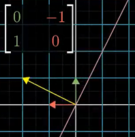
Not all transformations have eigenvectors. One example is a 2D 90° counterclockwise rotation which rotates all vectors off their spans as shown in Figure 4. Consider computing the eigenvalues of this rotation. Subtract λ from the diagonal elements and look for when the determinant is zero.

det([-λ -1]) = (-λ)(-λ) - -1*1 = 0
    [ 1 -λ]
             = λ² + 1 = 0

∴ λ = i or λ = -i

The only roots of that polynomial are the imaginary numbers i and -i. Assuming we are only looking for real number solutions, there are no eigenvectors for that transformation. However note that eigenvalues that are complex numbers generally correspond to some kind of rotation in the transformation.

Whenever a matrix has zeroes everywhere other than the diagonal, it is called a diagonal matrix. The way to interpret this is that all the basis vectors are eigenvectors with the diagonal entries of the matrix being their eigenvalues. That is, a diagonal matrix simply scales the basis vectors. A diagonal matrix can be represented as a vector times the identity matrix I. For example:

Figure 5: Change of basis

[-1 0] = [1 0][-1]
[ 0 2]   [0 1][ 2]

Therefore, whenever we want to apply a matrix multiplication to a diagonal matrix, it is the same as applying a matrix-vector multiplication, converting an O(N²) operation into O(N).

If a transformation has enough eigenvectors such that you can choose a set that spans the full space, then you can change your coordinate system so that these eigenvectors are your basis vectors. For example, using the eigenvectors for the matrix from Figure 1 as the change of basis matrix (the green and yellow arrows):

[1 -1]^-1[3 1][1 -1] = [3 0]
[0  1]  [0 2][0  1]   [0 2]

This new matrix is guaranteed to be diagonal with its corresponding eigenvalues down that diagonal. The new basis is called an eigenbasis with Figure 5 showing the change of basis. Applying the transformation will scale the new basis vectors by those eigenvalues, that is, the green arrow by 3 and the yellow arrow by 2.

Next up: vector spaces

--

[1] The figures and examples of the posts in this series are based on the Essence of Linear Algebra series by 3Blue1Brown.

[2] A vector that remains on its span either points in the same direction or points in the opposite direction (the negative direction).